Multiple Choice
Identify the choice that best
completes the statement or answers the question.
|
|
|
1.
|
Use a ruler to help you estimate the y-intercept for a line that best
approximates the data in the scatter plot. 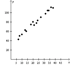
|
|
|
2.
|
Determine the equation of the quadratic regression function for the data.
x | 1 | 2 | 3 | 4 | 5 | y | 100.8 | 101.3 | 101.5 | 100.9 | 99.8 | | | | | | |
A. | y = –0.3x2 + 1.5x + 99.6 | B. | y =
–1.3x2 + 0.5x + 99.6 | C. | y =
–0.5x2 + 1.3x + 99.6 | D. | y =
–1.5x2 + 0.3x + 99.6 |
|
|
|
3.
|
Match the following graph with its function. 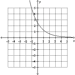
|
|
|
4.
|
Match the following graph with its function. 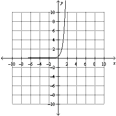
A. | y = – ln x ln x | B. | y = 3 log x | C. | y =
– (3)x (3)x | D. | y =
0.3(10)x |
|
|
|
5.
|
The equation of the logarithmic function that models a data set is y =
43.9 – 8.7 ln x.
Interpolate the value of y when x = 5.5.
A. | y = 23 | B. | y = 25 | C. | y =
27 | D. | y = 29 |
|
|
|
6.
|
The following data set involves logarithmic growth. Determine the missing
value. x | 1 | 5 | 10 | 20 | 50 | 100 | y | 0.0 | 0.7 | 1.0 | 1.3 | 1.7 | | | | | | | | |
|
|
|
7.
|
Determine the equation of the logarithmic regression function for the
data. x | 1 | 2 | 3 | 4 | 5 | 6 | y | 0.0 | 3.2 | 4.5 | 5.0 | 5.4 | 5.6 | | | | | | | |
A. | y = 1.55 + 4.25 ln x | B. | y = 0.54 + 3.11 ln
x | C. | y = 2.74 + 1.31 ln x | D. | y = –0.81 + 2.45 ln
x |
|
|
|
8.
|
Choose the best estimate for 7 radians in degrees.
|
|
|
9.
|
Choose the best estimate for the central angle in radians. 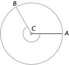
|
|
|
10.
|
Determine the amplitude of the following function.
y = 3 sin
2(x + 90°) – 1
|
|
|
11.
|
Determine the amplitude of the following function.
y = 0.5 sin
(x – 2)
|
|
|
12.
|
Determine the midline of the following function.
y = 0.5 sin (x
– 2)
A. | y = –2 | B. | y = 0.5 | C. | y =
0 | D. | y = 2 |
|
|
|
13.
|
The following data set is sinusoidal. Determine the missing value from the
table.
|
|
|
14.
|
Determine the equation of the sinusoidal regression function for the
data. x | 0 | 1 | 2 | 3 | 4 | 5 | 6 | 7 | y | –1.0 | 1.1 | 11.1 | 16.5 | 10.5 | 0.6 | –0.8 | 8.0 | | | | | | | | | |
A. | y = 7.4 sin (1.2x – 2.0) + 9.1 | B. | y = 7.4 sin
(1.2x – 2.0) – 9.1 | C. | y = 9.1 sin (1.2x – 2.0) +
7.4 | D. | y = 9.1 sin (1.2x – 2.0) –
7.4 |
|
|
|
15.
|
The amount of daylight in a town can be modelled by the sinusoidal function
d(t) = 4.37 cos 0.017t + 12.52
where d(t) represents the
hours of daylight and t represents the number of days since June 20, 2012.
How many hours
of daylight should be expected on August 20, 2012?
A. | 14.74 h | B. | 14.89 h | C. | 15.04
h | D. | 15.19 h |
|
Short Answer
|
|
|
1.
|
Determine if the exponential function h( x) =  is increasing
or decreasing.
|
|
|
2.
|
Sketch the exponential function f( x) =  .
|
|
|
3.
|
Determine the range of the following function. y =  cos ( x
– p)
|
Problem
|
|
|
1.
|
A hockey coach want to know the relationship between the number of shots his
team takes during a game and the number of goals they score. She collected the following data from
the last few games. Shots | 11 | 20 | 24 | 28 | 27 | 33 | 17 | 38 | Goals | 1 | 2 | 0 | 3 | 2 | 3 | 1 | 4 | | | | | | | | | |
a) Create a scatter plot, and draw a
line of best fit for the data. b) Use your graph to estimate the number of shots required
to score 3 goals.
|
|
|
2.
|
How can you use the graph of the function y = ex to
help you graph the function y = ln x? Include a diagram with your explanation.
|
|
|
3.
|
The following data can be modelled with a logarithmic function. x | 2 | 4 | 6 | 10 | 15 | 25 | 40 | y | 3.7 | 4.1 | 4.4 | 4.6 | 4.8 | 5.0 | 5.3 | | | | | | | | |
a) Create a scatter plot, and draw a curve of best fit for
the data using logarithmic regression. b) Use your graph to interpolate the y-value
when x = 32, to the nearest hundredth.
|